
Validation/Compressible flow
Sod shock tube
The exact Riemann solution, compared point by point. It found a defect nobody had noticed: the solver was using the wrong ratio of specific heats.
Why this case first
Almost every validation case in computational fluid dynamics compares a simulation against an experiment, and an experiment carries its own error bars. This one does not. A tube of gas with a discontinuity in it has a closed-form answer — the Riemann problem for the Euler equations — so the comparison is against arithmetic, and any disagreement is ours.
That makes it the first case to run and the hardest to argue with.
| Physics | Compressible, inviscid, one-dimensional |
|---|---|
| Solver | Density-based, central-upwind (Kurganov–Tadmor) |
| Reference | Exact Riemann solution — Toro, Riemann Solvers and Numerical Methods for Fluid Dynamics, 3rd ed., ch. 4 |
| Agreement | L1 error 0.084 % to 0.166 % of range on 1000 cells |
| Reproduce | Worked examples → Sod shock tube (validation) → Generate mesh → Run |
The problem
A tube ten metres long, closed at both ends, divided by a diaphragm at the middle. The gas on the left is at ten times the pressure and eight times the density of the gas on the right, and both are at rest.
Initial states
        x = -5 m                    0                      x = +5 m
        ┌───────────────────────────┬───────────────────────────┐
        │   p = 100 kPa             │   p = 10 kPa              │
        │   T = 348.432 K           │   T = 278.746 K           │
        │   ρ = 0.99965 kg/m³       │   ρ = 0.12496 kg/m³       │
        │   u = 0                   │   u = 0                   │
        └───────────────────────────┴───────────────────────────┘
                              diaphragm
At t = 0 the diaphragm is removed. Three waves result, and they are the whole of the answer: a shock running right into the low-pressure gas, a contact surface behind it, across which density and temperature jump but pressure and velocity do not, and an expansion fan running left into the high-pressure gas.
The gas is air: molecular weight 28.96, so R = 287.10 J/kg·K, with a constant Cp of 1004.5 J/kg·K giving γ = 1.4003.
The governing equations
The one-dimensional Euler equations — conservation of mass, momentum and total energy, with no viscosity and no conduction:
    ∂ρ/∂t    +  ∂(ρu)/∂x        =  0
    ∂(ρu)/∂t +  ∂(ρu² + p)/∂x   =  0
    ∂E/∂t    +  ∂(u(E + p))/∂x  =  0
closed by the ideal gas law and the definition of total energy:
p = ρRT E = p/(γ−1) + ½ρu²
The exact solution
The pressure in the region between the two waves, p*, is the root of
f_L(p) + f_R(p) + (u_R − u_L) = 0
where each f is the jump condition for whichever wave that side turns out to be — a shock if p > p_k, an expansion if p < p_k:
    shock       f_k = (p − p_k) √[ A_k / (p + B_k) ]
                A_k = 2 / ((γ+1) ρ_k)       B_k = p_k (γ−1)/(γ+1)

    expansion   f_k = (2a_k /(γ−1)) [ (p/p_k)^((γ−1)/2γ) − 1 ]
Solved by Newton iteration, the star state for this problem is
| Quantity | Value |
|---|---|
| p* | 30 313 Pa |
| u* | 293.34 m/s |
| ρ* left of the contact | 0.42617 kg/m³ |
| ρ* right of the contact | 0.26548 kg/m³ |
| T* left of the contact | 247.75 K |
| T* right of the contact | 397.71 K |
and the waves travel at
| Wave | Speed | Position at t = 0.007 s |
|---|---|---|
| Expansion head | −374.23 m/s | x = −2.620 m |
| Expansion tail | −22.23 m/s | x = −0.156 m |
| Contact surface | +293.34 m/s | x = +2.053 m |
| Shock | +554.18 m/s | x = +3.879 m |
Our set-up
| Domain | 10 m × 0.01 m × 0.01 m |
|---|---|
| Mesh | 1000 × 1 × 1 uniform cells, 10 mm |
| Sides | Symmetry planes — one-dimensional in everything but the mesh |
| Ends | Walls, unreached at the time compared |
| Time | To t = 0.007 s, step adjusted to hold Courant 0.2 |
| Cores | 1 |
| Output | ASCII, so the numbers can be read directly |
Nothing is set up outside the product: the case is a worked example, and the initial states are applied with the same region-fill any user has.
Results
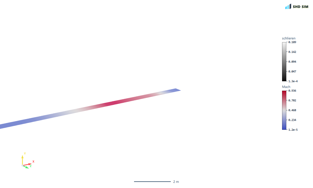
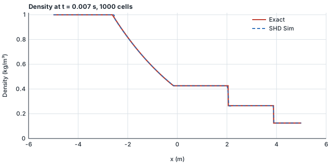
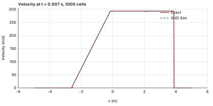
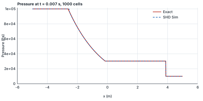
The expansion fan, the plateau, the contact and the shock all sit where the exact solution puts them. The two curves are hard to tell apart except at the discontinuities, which is where a finite mesh must smear a jump over a few cells.
| Field | L1 | L∞ | L1 as % of range | L∞ as % of range |
|---|---|---|---|---|
| Density | 8.61 × 10⁻⁴ kg/m³ | 0.0722 kg/m³ | 0.098 % | 8.26 % |
| Velocity | 0.486 m/s | 124.2 m/s | 0.166 % | 42.3 % |
| Pressure | 75.3 Pa | 6173 Pa | 0.084 % | 6.86 % |
Mesh refinement
One agreeing result is not verification — it is one number that happens to be close. What makes it verification is that the error falls when the mesh is refined, at a rate the scheme is supposed to give.
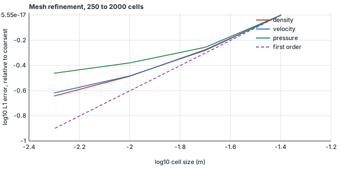
| Cells | Cell size | L1 density | L1 velocity | L1 pressure |
|---|---|---|---|---|
| 250 | 40 mm | 2.638 × 10⁻³ | 1.480 | 180.6 |
| 500 | 20 mm | 1.401 × 10⁻³ | 0.776 | 100.2 |
| 1000 | 10 mm | 8.611 × 10⁻⁴ | 0.486 | 75.3 |
| 2000 | 5 mm | 5.998 × 10⁻⁴ | 0.356 | 62.3 |
| Meshes | Density | Velocity | Pressure |
|---|---|---|---|
| 250 → 500 | 0.91 | 0.93 | 0.85 |
| 500 → 1000 | 0.70 | 0.68 | 0.41 |
| 1000 → 2000 | 0.52 | 0.45 | 0.27 |
The observed order starts near one and falls towards a half, which is the expected behaviour for a shock-capturing scheme on this problem rather than a shortcoming: a second-order scheme is reduced to first order at a discontinuity, and the contact surface — which has no self-steepening mechanism to hold it together — smears as the square root of time, so its contribution to the error falls more slowly still. A scheme that reported second order here would be one that was not resolving the contact.
What the remaining difference is
Discretisation, and specifically the capture width of the two discontinuities. The error is concentrated within a few cells of the shock and the contact; in the smooth regions — the undisturbed gas at each end, the plateau, the interior of the expansion — it is at the level of round-off. Refining the mesh narrows the capture and the error falls with it.
What this case found
It is worth saying plainly that this page exists because the case caught something.
Before this comparison was made, the solver was being handed a thermophysical package written in terms of enthalpy. A density-based solver works in internal energy, and given the wrong one it used the constant labelled Cp where Cv belongs — so it was running with
γ = (Cp + R) / Cp = 1.2858 instead of Cp / (Cp − R) = 1.4003
Eight per cent wrong in the ratio of specific heats, in a solver whose whole subject is compressible waves. Every case ran to completion, wrote its fields and opened for post-processing, and every number in them was the answer for a slightly different gas.
What exposed it was not the disagreement itself — 1.7 % in the star pressure looks like a mesh effect — but that the error did not fall when the mesh was refined, on any of four meshes from 250 to 2000 cells. An error that does not refine away is not a discretisation error. Solving the same Riemann problem for γ = 1.286 lands on the numbers we were getting.
The figures and tables above are from the corrected solver.
Reproducing this
- Worked examples → Sod shock tube (validation)
- Generate mesh, then Run
- Compare against the exact solution, which is computed from the equations above rather than transcribed from a table — so there is no reference data to mistype and nothing to take on trust.
Repeat this yourself
Every case here is set up from the worked examples in the product, with no hand-editing of solver files — so you can run it, and get the same numbers. The free tier runs real cases up to 250,000 cells of fluids, or 100,000 nodes of solid, with no account needed to download and no time limit.
All validation cases · Written by the team building SHD Sim.