
Validation/Acoustics
The notes a closed duct plays
A rigid tube’s resonances are n·c/2L exactly. Driving it with a moving piston rather than a pressure exercises a different path through the solver from the duct-resonance case.
Why this case
A rigid-walled tube of length L closed at both ends has the plane-wave eigenfrequencies
f_n = n c / (2 L), n = 1, 2, 3, ...
exactly. The c here is the c the case hands the solver — 343.0 m/s, the application’s own default for air — rather than a constant looked up elsewhere. √(γRT) at 20 °C is 343.23, which is close and is deliberately not the reference: the arithmetic is on the case’s own inputs, so there is nothing in it to mis-transcribe and no experiment to argue about.
This is not a repeat of the existing duct-resonance case. That one states a pressure at one end, which is a Dirichlet condition, so its poles are at the quarter-wave frequencies; and it measures an amplification at a fixed 1000 Hz rather than a frequency at all. This one drives the duct with a piston — a normal velocity — which the deck writer turns into a wave flux on the imaginary part, and it measures a frequency. Different boundary-condition code path, different arithmetic.
| Physics | Harmonic acoustics, Helmholtz equation, rigid-walled duct |
|---|---|
| Geometry | A 0.1 m duct, 0.02 m across |
| Mesh | 1 383 tetrahedra, 2 776 points, maxh 0.005 m |
| Air | ρ = 1.225 kg/m³, c = 343.0 m/s |
| Drive | Normal velocity 0.01 m/s at one end; every other surface rigid |
| Reference | f₁ = 1715 Hz, f₂ = 3430 Hz, ratio exactly 2 |
| Agreement | Both eigenfrequencies within 0.0014 % |
| Last run | 2026-08-27 |
How a closed duct is driven at all
Both ends rigid is an eigenvalue problem and it has no forced answer: with no drive the cavity solves to silence. So one end becomes a piston, and everything else is left rigid — which is the Helmholtz equation’s natural boundary and needs no condition stated. The exact response is then
p(x) = i rho c v cos(k (L - x)) / sin(k L), k = omega / c
whose poles are exactly sin(kL) = 0, that is kL = nπ, that is f = n·c/2L. Driving the duct does not move its resonances; it only makes them visible.
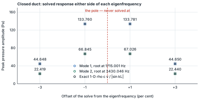
Nothing is ever solved at a resonance. With no losses in the Helmholtz equation the amplitude there is infinite, and the numerical answer would be whatever the nearly singular linear system happened to return. Sweeping for a peak would measure the sweep’s own step size. Instead each resonance is found as the root of the reciprocal amplitude — 1/|p| = |sin kL| / (ρcv) is a straight line through zero at the resonance — by a secant through one well-conditioned solve each side of it.
Result
| Quantity | Measured | Reference | Difference |
|---|---|---|---|
| f₁ | 1715.001342 Hz | 1715 Hz | +0.000078 % |
| f₂ | 3430.046352 Hz | 3430 Hz | +0.001351 % |
| f₂ / f₁ | 2.0000255 | exactly 2 | +0.001273 % |
The ratio is the check with no escape, and it is the reason both modes are run. f₁ on its own is dominated by c and L, which are both inputs — a deck faithfully carrying a wrong speed of sound would still be perfectly self-consistent, and so would a mis-scaled geometry. The ratio cancels c, it cancels L, it cancels the density and the piston amplitude. What is left is only whether the discrete operator has the dispersion relation of the wave equation.
| Guard | Worst measured | What it establishes |
|---|---|---|
| Off-resonance amplitude | 0.163 % | The 3-D field being extrapolated from is the 1-D standing wave the reference describes |
| Divergence ratio | 0.000123 % | A pole is actually between the sampling points |
| Span drift | 6.32 × 10⁻⁷ | Each root measured twice, from a ±1 % pair and a ±3 % pair, agrees with itself |
| Transverse spread | 5.61 × 10⁻⁴ of the peak | The field is a plane wave, so a one-dimensional reference applies to it |
The frequency measurement is not self-validating
The divergence ratio is the sharpest of the four. |p| goes as 1/|f − fn| near a pole, so the amplitude at ±1 % must exceed the amplitude at ±3 % by very nearly three — the harness computes the exact ratio rather than assuming 3, and gets 2.99605330 against an exact 2.99605346 on the first mode. On the deck with no pole there it comes out 0.99.
What a mesh too coarse looks like
A third companion run takes the same duct on 30 tetrahedra instead of 1 383. The frequencies do not collapse — f₁ comes back at +0.0073 % and f₂ at +0.111 % — but the errors are one to two orders of magnitude larger than on the mesh above, and they grow with mode number, which is exactly the dispersion behaviour a finite element has. The transverse spread goes to 3.80 × 10⁻² of the peak, so the field is no longer a plane wave, and the one-dimensional reference no longer describes what was solved.
That is the useful shape of the failure: the frequency drifts a little, and the statement that a one-dimensional reference applies at all stops being true first.
Repeat this yourself
Every case here is set up from the worked examples in the product, with no hand-editing of solver files — so you can run it, and get the same numbers. The free tier runs real cases up to 250,000 cells of fluids, or 100,000 nodes of solid, with no account needed to download and no time limit.
Other cases
- Duct resonanceA closed form for the resonant frequency, and a mesh sweep that converges onto it monotonically.
- A pressure wave crossing a tubeA wave that stays smooth, so the answer is exact for as long as it does. It is also the case that showed refining the mesh alone can hide a first-order time scheme completely.
All validation cases · Written by the team building SHD Sim.