
Validation/Compressible flow
A pressure wave crossing a tube
A wave that stays smooth, so the answer is exact for as long as it does. It is also the case that showed refining the mesh alone can hide a first-order time scheme completely.
Why a smooth wave, alongside the shock tube
Not because a Riemann problem cannot verify this family. It can — at converged correctors the pressure-based compressible solver reproduces the exact star velocity to −0.01 %.
A smooth wave earns its place on its own merits. It is the regime this family is actually sold for — transient heating, compressible pulsation, valve and manifold flow — and, having no discontinuity in it, it isolates what a shock tube cannot: the scheme’s own dispersion and damping, read directly as where the pulse has got to and how tall it still is, with no limiter or capturing behaviour in the way.
It is also the only regime here in which an error can be made to fall at a rate, because a solution with a discontinuity in it has no order to measure.
| Physics | Transient, compressible, one-dimensional; pressure-based solver |
|---|---|
| Tube | 10 m, meshed 500, 1000 and 2000 cells along |
| Undisturbed state | p₀ = 100 000 Pa, T₀ = 300 K, γ = 1.4, so c₀ = 347.2733793 m/s |
| Pulse | A smooth Gaussian, 200 Pa tall — 0.2 % of ambient — half-width 0.5 m |
| Time | To 0.004 s, about 1.4 m of travel |
| Solver settings | 50 outer correctors; linear tolerance 10⁻¹², relative tolerance 0 |
| Reference | The exact simple wave; Riemann invariants, after Whitham, Linear and Nonlinear Waves |
| Agreement | Wave speed within 0.06 %; observed order 1.03 refining space and time together |
The reference is exact, not linearised
A right-running simple wave has the Riemann invariant
J- = u - 2c/(gamma-1)
constant everywhere, which fixes the velocity belonging to a given pressure:
u = 2 c0/(gamma-1) * ( (p/p0)^((gamma-1)/(2 gamma)) - 1 )
and then every point of the profile travels at its own speed u + c, so
x(x0, t) = x0 + ( u0 + c0 + (gamma-1)/2 * u0 ) * t
which is exact for smooth flow, at any amplitude, until neighbouring characteristics cross and a shock forms. This is not acoustics with the nonlinear terms dropped: the wave really does steepen over the run, and the reference steepens with it. That is why the exact peak position and the exact peak height in the table below differ slightly from mesh to mesh — they are evaluated at each run’s own sampling.
Result
Three things are measured on each of three meshes.
- Where the pulse is — its speed, which is the physics
- How tall it still is — numerical damping, which is the scheme
- L1 against the exact profile, which is everything at once
| Cells | Time step | Speed (m/s) | Exact (m/s) | vs exact | Peak height (Pa) | vs exact |
|---|---|---|---|---|---|---|
| 500 | 2 × 10⁻⁶ s | 347.65625 | 347.86709 | −0.061 % | 199.15 | −0.424 % |
| 1000 | 1 × 10⁻⁶ s | 347.83333 | 347.86828 | −0.010 % | 199.60 | −0.195 % |
| 2000 | 5 × 10⁻⁷ s | 347.81250 | 347.86877 | −0.016 % | 199.82 | −0.089 % |
Refining the mesh alone says nothing
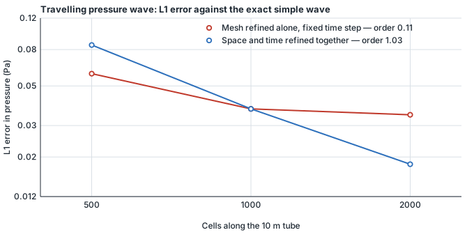
This is the part of the case worth keeping, and it is why the observed order on this page is 1.03 rather than 2.
| Cells | L1 — mesh refined alone, step held at 10⁻⁶ s | L1 — space and time refined together |
|---|---|---|
| 500 | 5.860528 × 10⁻² | 8.480622 × 10⁻² |
| 1000 | 3.719926 × 10⁻² | 3.719926 × 10⁻² |
| 2000 | 3.447622 × 10⁻² | 1.821669 × 10⁻² |
| Meshes | Mesh refined alone | Space and time together |
|---|---|---|
| 500 → 1000 | 0.656 | 1.189 |
| 1000 → 2000 | 0.110 | 1.030 |
The fixed-step study stalls, and the cause is the time scheme: the case integrates with Euler, which is first order in time. A fixed step therefore contributes an error the mesh cannot refine away, and the observed order collapses onto that floor.
That was identified rather than guessed at, by halving the step at a fixed mesh, where the error does move: at 500 cells the L1 goes from 8.480622 × 10⁻² at a step of 2 × 10⁻⁶ s to 5.860528 × 10⁻² at 10⁻⁶ s. So the study halves the step as the cell count doubles, holding the Courant number constant. Space and time then refine together, and 1.03 is the right answer: it is what the slower of a second-order space and a first-order time discretisation must give.
Two of the product's own defaults had to be changed
Both are reported here rather than quietly applied, because each was in turn the thing limiting this measurement — and both are what a user gets if they do not change them.
What this page does not establish
- The order is 1.03, and that is a first-order result. It is the correct order for this scheme combination, not a good one. Anybody wanting second order in time needs a different time scheme, and this page has not run one.
- Nothing here is a mesh study. Refining the mesh alone floors at 0.110 on this case, and a page reporting only that would have shown a converged-looking result that meant nothing. The two studies are shown side by side for exactly that reason.
- The settings above are not the product’s defaults. Every number on this page is at 50 outer correctors and tightened linear tolerances. Run with what the product writes, this case is about 11 % slow, and the section above says so with its own table.
- The wave is smooth, and that is the whole point. Once characteristics cross the reference stops being exact. Nothing on this page says anything about how this solver handles a discontinuity — that is what the shock tube case is for.
Repeat this yourself
Every case here is set up from the worked examples in the product, with no hand-editing of solver files — so you can run it, and get the same numbers. The free tier runs real cases up to 250,000 cells of fluids, or 100,000 nodes of solid, with no account needed to download and no time limit.
Other cases
All validation cases · Written by the team building SHD Sim.