
Validation/Eddy currents
Eddy-current loss in an AC bar
A square bar in its own alternating field has no closed-form loss. The low-frequency asymptotic is exact for any shape, and the mesh cancels out of it.
Why this case
A copper bar one metre long and 20 mm square, carrying 100 A, in an air region, at four frequencies from 1 Hz to 16 Hz. The alternating current induces currents in the conductor’s own body, and those currents dissipate.
A square bar in its own alternating field has no closed-form loss. Saying so is the starting point of this page, because it decides what can honestly be measured.
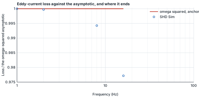
What is exact — and exact for any geometry whatsoever — is the low-frequency asymptotic. The induced electric field is −iωA, the induced current density is σ times that, and the dissipation goes as its square:
- P ∝ ω², so P(2f) / P(f) → 4
Every geometric factor lives in the constant and cancels in the ratio. So does the mesh, so does the air region, and so does the domain truncation — numerator and denominator are the same solve at a different frequency.
| Physics | Harmonic magnetics with induced currents |
|---|---|
| Material | Annealed copper, σ = 5.96 × 10⁷ S/m, non-magnetic |
| Applied | 100 A total, at 1, 2, 8 and 16 Hz |
| Closed form | The low-frequency asymptotic P ∝ ω², so P(2f)/P(f) = 4 |
| Mesh | Tetrahedral with an air region — 52 929 mesh points |
| Agreement | 3.9989 against an exact 4 at the low pair |
| Last run | 2026-08-27 |
Result
| Frequency | Skin depth | Joule loss (W) | Ratio to the previous |
|---|---|---|---|
| 1 Hz | 0.0652 m | 4.399088 × 10⁻⁶ | — |
| 2 Hz | 0.0461 m | 1.759151 × 10⁻⁵ | 3.9989 |
| 8 Hz | 0.0230 m | 2.799251 × 10⁻⁴ | 15.9125 |
| 16 Hz | 0.0163 m | 1.100452 × 10⁻³ | 3.9312 |
The measurement is the 1 Hz to 2 Hz ratio: 3.9989 against an exact 4, which is −0.028 %.
The field, as a second check
At the lowest frequency the field must still be the magnetostatic one, so it has to come back at Ampère’s law — the same comparison, on the same geometry, as the straight-conductor case.
| Radius | Measured |B| (T) | Ampère (T) | Difference |
|---|---|---|---|
| 0.0573 m | 3.209027 × 10⁻⁴ | 3.488332 × 10⁻⁴ | −8.007 % |
| 0.0832 m | 2.455667 × 10⁻⁴ | 2.403962 × 10⁻⁴ | +2.151 % |
That is the magnetostatic page’s own band on this air mesh, and it comes from domain truncation rather than from the physics. It is here as a check that the right equation is being solved. The ratio is the precision measurement.
What the ratio catches, and what it does not
The automated check that guards this case is tested against a deck with the conductor’s conductivity left out. That deck reports a loss of exactly zero at every frequency — which is the arithmetically correct answer to a model with nothing to induce in.
Its magnetic field is identical to the healthy run’s to every digit, because removing the conductivity does not change the field equation at all, only the term that dissipates. The Ampère comparison above passes on it and says nothing. That is why the loss is judged and not only the field.
Repeat this yourself
Every case here is set up from the worked examples in the product, with no hand-editing of solver files — so you can run it, and get the same numbers. The free tier runs real cases up to 250,000 cells of fluids, or 100,000 nodes of solid, with no account needed to download and no time limit.
Other cases
- Straight conductor, against AmpèreAmpère’s law is exact and the geometry is trivial, which is what makes the residual difference worth reporting rather than explaining away.
- DC conduction through a barThe potential in this problem does not depend on the conductivity at all, so a deck that lost it entirely would still give a perfect voltage field. The derived fields are the measurement.
All validation cases · Written by the team building SHD Sim.