
Validation/Buoyancy and heat transfer
Natural convection in a heated cavity
The only case here where the flow is caused by the temperature field rather than imposed on it — and the one that showed “converged” is a claim about residuals.
Why this case
A square box of air, one wall hot and the opposite wall cold, the other two insulated. Nothing stirs it. The air near the hot wall expands, becomes lighter than the air around it, rises, crosses the top, cools against the far wall and sinks — and that circulation is the whole of the flow.
Every other case in this section imposes the flow and then asks what the fluid does with it. This one has no inlet and no moving surface. The velocity field is an output of the temperature field, which means momentum and energy have to be solved together and the coupling between them is the thing under test. If the buoyancy term is scaled wrongly, or the two equations are advanced out of step, there is no imposed flow to hide behind: the circulation is simply the wrong strength.
It is also the case where the answer is a single heat-transfer number rather than a profile. The average Nusselt number on the hot wall is how much heat crosses it compared with conduction alone, so it is the ratio the whole simulation exists to predict.
The governing parameter
Ra = g·β·ΔT·L³ / (ν·α)        α = ν / Pr

  g   gravity                    β   thermal expansion coefficient
  ΔT  hot wall − cold wall       L   cavity side
  ν   kinematic viscosity        α   thermal diffusivity, Pr = 0.71 for air
Rayleigh number is the ratio of buoyancy driving the flow to the viscosity and conduction damping it. At 10⁴ the circulation is a single slow cell; by 10⁶ it has thinned into boundary layers up the two vertical walls with a nearly stagnant stratified core between them. Running all three decades tests the same physics at three quite different regimes.
| Physics | Incompressible, laminar, Boussinesq buoyancy, steady |
|---|---|
| Rayleigh number | 10⁴, 10⁵ and 10⁶, at Pr = 0.71 |
| Reference | Wan, D.C., Patnaik, B.S.V., Wei, G.W., A New Benchmark Quality Solution for the Buoyancy-Driven Cavity by Discrete Singular Convolution |
| Agreement | Average Nusselt number within 1.6 % of the reference’s finite element result at every Rayleigh number |
| Mesh | 40 × 40, 80 × 80 and 160 × 160 — nine runs in all |
| Reproduce | Worked examples → Buoyant cavity (example), then set it two-dimensional, walls to 307.75 K and 288.15 K, and the box to 38.184 mm for Ra = 10⁵. There is no one-click preset for this one yet |
The reference
The canonical citation for this benchmark is de Vahl Davis (1983), and it is not the one used here. It is paywalled, with no public data file, and it is reproduced in dozens of later papers — none of which is a sound source for it. A reference column has to come from a paper we have read, reporting what that paper itself computed. Quoting a table that quotes a table is how a transcription error outlives everybody who could have caught it.
Wan, Patnaik and Wei solve the same cavity by two completely independent numerical procedures — a discrete singular convolution scheme and a Galerkin finite element method — and tabulate both. Citing a paper for its own results is sound, and two independent methods are a stronger reference than one.
Result
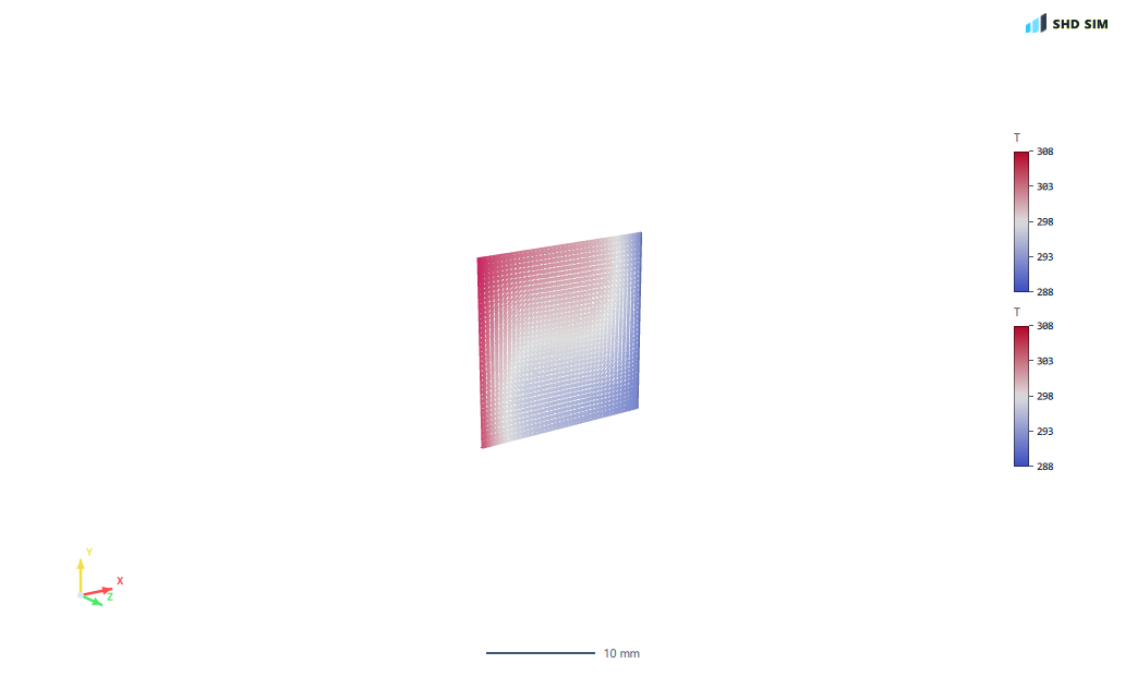
Average Nusselt number on the hot wall. Each run is 60 000 iterations, and each was checked for stillness at the end rather than stopped when a residual fell — for the reason below.
| Ra | mesh | SHD Sim | vs FEM | vs DSC |
|---|---|---|---|---|
| 10⁴ | 40 × 40 | 2.2596 | +0.25 % | +4.85 % |
| 10⁴ | 80 × 80 | 2.2484 | −0.25 % | +4.33 % |
| 10⁴ | 160 × 160 | 2.2466 | −0.33 % | +4.25 % |
| 10⁵ | 40 × 40 | 4.6418 | +0.95 % | +6.66 % |
| 10⁵ | 80 × 80 | 4.5479 | −1.09 % | +4.50 % |
| 10⁵ | 160 × 160 | 4.5286 | −1.51 % | +4.06 % |
| 10⁶ | 40 × 40 | 9.8272 | +9.48 % | +13.85 % |
| 10⁶ | 80 × 80 | 9.0233 | +0.53 % | +4.53 % |
| 10⁶ | 160 × 160 | 8.8685 | −1.20 % | +2.74 % |
At all three Rayleigh numbers the finest mesh sits inside the band between the two reference methods — 2.2466 against their 2.155 and 2.254, 4.5286 against 4.352 and 4.598, and 8.8685 against 8.632 and 8.976. Ours is nearer the finite element solution at every decade, and at none of them is it outside the spread the reference has with itself.
The refinement study is the real result
Agreeing with a published number on one mesh is weak evidence — a coarse mesh and a compensating error land on the right answer often enough to be untrustworthy. What cannot be faked is the way the answer moves as the mesh is refined.
With a uniform refinement ratio of two, the successive changes give the observed order of accuracy directly:
Observed order of accuracy
p = log₂( |N₈₀ − N₄₀| / |N₁₆₀ − N₈₀| )

  Ra = 10⁴    |−0.0112| , |−0.0018|    →   p = 2.64
  Ra = 10⁵    |−0.0939| , |−0.0193|    →   p = 2.28
  Ra = 10⁶    |−0.8039| , |−0.1548|    →   p = 2.38
All three come out near two, which is what the discretisation claims to be, and the changes shrink by a factor of five to six each time the mesh is halved — at every Rayleigh number, across three decades and a factor of four in the answer itself. That is a statement about the code alone; it needs no reference paper at all, and it is the part of this page that would survive if the benchmark values were withdrawn tomorrow.
What this case found
The first attempt at this benchmark produced numbers that got worse under refinement. At Ra = 10⁵ the three meshes gave 4.674, 4.790 and 5.217: the steps were growing, where a mesh-converged quantity’s must shrink, and every value sat above both reference methods and moved further above them as the mesh improved.
A benchmark that disagrees is publishable. One whose own refinement study is diverging is not, because there is no limit to quote. The cause turned out not to be the physics.
One candidate was eliminated rather than assumed. The first runs had the default k-ω SST turbulence model left on, which would have been a genuine setup error for a laminar benchmark — but re-running laminar moved Nu at Ra = 10⁵ from 4.6740 to 4.6742. The eddy viscosity was already negligible, so the model was never the cause, and saying so is worth more than quietly fixing it and taking the credit.
What this case does not cover
- The Boussinesq approximation. Density is taken as constant everywhere except in the buoyancy term. That is standard for this benchmark and sound for small temperature differences, but it is an approximation this case cannot test, because the reference makes it too.
- Turbulent natural convection. All three Rayleigh numbers here are laminar. Real buoyant flows in rooms and enclosures run several decades higher, where the boundary layers become unsteady and a turbulence model starts to matter.
- Conjugate heat transfer. The walls are boundary conditions, not solids. Nothing here tests conduction through a wall into the fluid, which is what most thermal work actually needs.
- Radiation. Excluded entirely. Above a few hundred kelvin it is often the dominant mode, and this case says nothing about it.
- Meshing. A uniform square block with no geometry in it — see the plate with a hole for a case where the mesh has to resolve a shape.
Repeat this yourself
Every case here is set up from the worked examples in the product, with no hand-editing of solver files — so you can run it, and get the same numbers. The free tier runs real cases up to 250,000 cells of fluids, or 100,000 nodes of solid, with no account needed to download and no time limit.
Other cases
- Lid-driven cavityThe oldest benchmark in incompressible CFD, run on a deliberately coarse mesh — because one that only agrees when it is expensive is not much of a reassurance.
- Turbulent plane channelThe only case here that tests turbulence modelling, against a DNS rather than an experiment — and it measures what a badly placed first cell costs you.
All validation cases · Written by the team building SHD Sim.