
Validation/Turbulence modelling
Turbulent plane channel
The only case here that tests turbulence modelling, against a DNS rather than an experiment — and it measures what a badly placed first cell costs you.
Why this case
Every other case on this site is laminar where it matters. The shock tube is inviscid, the plate is a solid, and neither says anything about the modelling decision that dominates real CFD: what happens between a wall and the first cell centre.
Fully developed flow between two parallel plates is the simplest wall-bounded turbulent flow there is — statistically one-dimensional, no pressure gradient along the wall, no curvature, no separation. That is exactly why it is the reference case. Any disagreement is attributable to the near-wall treatment, because there is nothing else it could be.
Moser, Kim and Mansour resolved it directly, with no turbulence model at all, and published the profiles. A direct numerical simulation is not a measurement, but for this flow it is better than one: it gives every statistic at every height, including quantities that are extremely hard to measure inside the viscous sublayer.
| Physics | Incompressible, fully developed, statistically 1-D |
|---|---|
| Solver | One-dimensional channel, steady, RANS |
| Reference | Moser, R.D., Kim, J., Mansour, N.N. (1999), Physics of Fluids 11(4) 943–945 — the Reτ = 392.24 dataset |
| Agreement | RMS error 0.341 in u+; centreline within 0.20 % |
| Reproduce | Pin boundaryFoam, set the target velocity and cell count, Run |
The reference, and reading it correctly
The dataset is published by its authors and can be downloaded from the Oden Institute’s turbulence database. The comparison below uses the mean-velocity and Reynolds-stress files, fetched from there rather than copied out of any secondary reproduction.
Two checks on the transcription, both of which the data passes: the wall row is exactly zero, as no-slip requires; and the first point sits in the viscous sublayer where u+ = y+ should hold, with 1.0605 against 1.0628 — agreement to 0.2 %.
Set-up
| Domain | Half-height 50 mm; one cell along the flow and across the span |
|---|---|
| Walls | No-slip, top and bottom |
| Streamwise faces | Periodic — the flow is fully developed by construction |
| Fluid | Air, ν = 1.51 × 10⁻⁵ m²/s |
| Mesh | Uniform, ungraded — so the first cell centre sits at exactly y+ = Reτ/N for N cells |
| Driving force | A body force adjusted to hold the target mean velocity |
| Achieved Re_τ | 395.81 on k-omega SST (+0.91 %), 392.04 on Spalart-Allmaras (−0.05 %) |
The ungraded mesh is not laziness, it is the instrument. Because the cells are uniform, one integer moves the first cell centre anywhere from the middle of the logarithmic region down into the viscous sublayer, which is what turns the usual advice about y+ into a measurement.
Result — the mean velocity profile
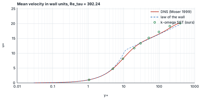
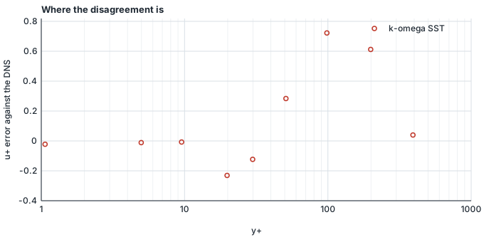
| y+ | DNS u+ | SHD Sim u+ | difference |
|---|---|---|---|
| 1.06 | 1.0605 | 1.0383 | −0.022 |
| 4.98 | 4.8032 | 4.7919 | −0.011 |
| 9.53 | 8.1754 | 8.1681 | −0.007 |
| 19.80 | 11.9660 | 11.7352 | −0.231 |
| 29.86 | 13.4790 | 13.3558 | −0.123 |
| 50.96 | 14.9020 | 15.1856 | +0.284 |
| 98.40 | 16.4930 | 17.2154 | +0.722 |
| 198.91 | 18.5350 | 19.1471 | +0.612 |
| 392.24 | 20.1330 | 20.1727 | +0.040 |
The sublayer and the buffer layer are reproduced almost exactly — three stations below y+ = 10 agree to better than 0.03 in u+. The largest disagreement is in the outer layer, and the centreline, which accumulates every error below it, lands within 0.20 %.
| Model | Re_tau reached | RMS in u+ | Centreline u+ | vs DNS |
|---|---|---|---|---|
| k-omega SST | 395.81 (+0.91 %) | 0.341 | 20.173 | +0.20 % |
| Spalart-Allmaras | 392.04 (−0.05 %) | 0.164 | 19.789 | −1.71 % |
It is worth resisting the urge to pick a winner here. Spalart-Allmaras follows the profile more than twice as closely and reaches the target Reynolds number almost exactly; k-omega SST puts the centreline within a fifth of a per cent where the other is off by 1.7. A one-line summary of that table would lose the only thing it says.
Result — turbulent kinetic energy
| Quantity | y+ of the DNS peak | DNS | SHD Sim | difference |
|---|---|---|---|---|
| Peak k+ | 16.89 | 4.5684 | 2.1625 | −53 % |
Result — what a badly placed first cell costs
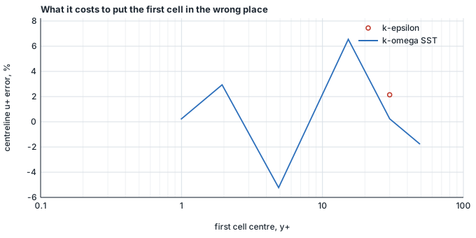
This is the measurement the case exists for. The near-wall treatment is valid in two places: resolved to the wall, with the first cell inside the viscous sublayer, or with the first cell out in the logarithmic region. In between — the buffer layer — neither assumption holds, and the usual advice is simply to avoid it.
Here is what ignoring that advice actually costs.
| Cells | First cell y+ | Centreline u+ | vs DNS 20.133 |
|---|---|---|---|
| 400 | 0.99 | 20.173 | +0.20 % |
| 200 | 1.94 | 20.724 | +2.94 % |
| 80 | 4.89 | 19.081 | −5.23 % |
| 26 | 15.25 | 21.451 | +6.55 % |
| 13 | 29.99 | 20.180 | +0.23 % |
| 8 | 49.22 | 19.776 | −1.78 % |
The error is smallest at the two placements where the treatment is valid — +0.20 % at y+ ≈ 1 and +0.23 % at y+ ≈ 30 — and worst in the buffer layer between them, reaching −5.2 % and +6.6 %. A five to seven per cent error in the centreline velocity, from nothing but where the first cell landed.
That is the number worth taking away from this page. It is not an argument that the software is accurate; it is an argument that a mesh which looks perfectly reasonable can cost several per cent, and that the only way to know is to check where your first cell sits.
What the wall treatment setting is worth
The mesh sweep above holds the near-wall treatment fixed and moves the mesh. This does the opposite: same mesh, same model, same target Reynolds number, and only the treatment changed.
| First cell | Treatment | RMS in u+ | Centreline error |
|---|---|---|---|
| y+ ≈ 1 | Wall functions | 0.341 | +0.20 % |
| y+ ≈ 1 | Automatic blending | 0.341 | +0.19 % |
| y+ ≈ 1 | Resolved (low-Re) | 0.341 | +0.19 % |
| y+ ≈ 30 | Wall functions | 0.551 | +0.23 % |
| y+ ≈ 30 | Automatic blending | 0.850 | −6.07 % |
| y+ ≈ 30 | Resolved (low-Re) | 16.251 | +78.6 % |
At y+ ≈ 1 the three are indistinguishable — identical to three decimal places. The blending function inside the model’s own transport equation already handles the near-wall region, and the log-law viscosity is negligible that close to a wall, so which form is written barely matters.
At y+ ≈ 30 they diverge sharply, and correctly. Asking for a resolved treatment on a mesh whose first cell sits out in the logarithmic region removes the modelled near-wall momentum transport, and the flow has to accelerate enormously to carry the same wall shear. A 79 % error in the centreline velocity is the right answer to the wrong question.
What this case found
Setting this benchmark up found three defects in our own software, and none of them was visible to a run that simply completed.
The one-dimensional channel solver was not solving its momentum equation at all. The faces normal to the flow were marked as a direction the solver does not solve in, so the streamwise velocity was never computed: it held its initial value for the entire run, giving a flat profile right up to a no-slip wall. The case reached its end time, wrote its fields, held its target flow rate exactly, and had been passing for months.
The wall treatment setting reached no case file. All three options produced identical conditions, so a user who meshed to y+ ≈ 1 and asked for a resolved treatment was getting a log-law wall function applied where its assumptions do not hold. That one was caught before any run — by noticing that the comparison table being prepared would have had three rows differing only in a label.
Spalart-Allmaras was broken twice over, and the convergence check refused to report a number for it both times rather than publishing one. Its modified viscosity was being set to the freestream value at no-slip walls instead of zero; correcting that took the driving gradient’s swing over the last two thousand iterations from 112.7 to 0.0034. It still would not settle, and the second cause was that the same quantity had no relaxation factor at all — the relaxation block named three turbulence variables and this was not one of them, so the equation ran completely unrelaxed while every other model ran at 0.7. With both corrected it converges in two attempts and gives the lowest profile error on this page.
What this case does not cover
- Separation. There is none and there cannot be. A model that reproduces this profile perfectly can still predict separation badly.
- Pressure gradients. The channel is fully developed with none along the wall — and adverse pressure gradients are where eddy-viscosity models actually differ from each other.
- Meshing. This is a graded block with no geometry in it. Nothing here validates the y+ that a surface mesher’s boundary layers actually achieve on a real body, which is the situation a user is in.
- High Reynolds number. Reτ = 392 is low. Behaviour at industrial Reynolds numbers is an extrapolation from this page, not a result on it.
Repeat this yourself
Every case here is set up from the worked examples in the product, with no hand-editing of solver files — so you can run it, and get the same numbers. The free tier runs real cases up to 250,000 cells of fluids, or 100,000 nodes of solid, with no account needed to download and no time limit.
Other cases
- Sod shock tubeThe exact Riemann solution, compared point by point. It found a defect nobody had noticed: the solver was using the wrong ratio of specific heats.
- Plate with a holeThe stress concentration factor of three, and a four-mesh study separating a coarse mesh from a finite plate — two explanations one run could not tell apart.
All validation cases · Written by the team building SHD Sim.