
Validation/Magnetohydrodynamics
A conducting fluid in a magnetic field
The magnetic field flattens the parabola into a plug with thin layers at the walls. The strong check is not the distance from the curve but the Hartmann number recovered from the measured shape.
Why this case
Magnetohydrodynamics was the one solver family in the product with no reference of any kind behind it. Its single solver was, until this case, only ever asked whether it reached End.
A conducting liquid flowing between two plates with a magnetic field applied across the channel has a closed-form profile, and the field does one specific thing to it: the parabola flattens into a plug with thin layers at the walls. That is what makes the case worth running. The parabola is what the same solver produces with the field switched off, so the question is not “does this produce a plausible channel profile” but “does the magnetic field do the one thing the arithmetic says it must”, at three separated field strengths.
| Physics | Laminar, incompressible, electrically conducting, with the full induction equation |
|---|---|
| Channel | Half-width a = 0.05 m, so 0.1 m across; 0.5 m long; 40 × 160 cells |
| Spanwise | Empty and one cell thick — infinite parallel plates, not a duct |
| Fluid | ρ = 1, ν = 1, μ = 1, σ = 0.001 in SI units; inlet 100 m/s |
| Field | B₀ = 0, 632.456, 3162.278 and 12 649.111, applied across the channel |
| Time | To 0.008 s at a fixed step of 3.902439 × 10⁻⁷ s |
| Reference | Hartmann (1937), Det Kgl. Danske Videnskabernes Selskab 15, 6 |
| Agreement | Hartmann number recovered from the measured shape: 1.0010256 and 5.0011318 against 1 and 5 |
The exact solution
Take a conducting liquid between plates at y = ±a, a uniform field B₀ applied across the channel, and let the flow become fully developed. Write the velocity as u(y) and the induced field as Bx(y). The steady induction equation reduces to
B0 u' + (1/(mu sigma)) Bx'' = 0 (1)
and the streamwise momentum equation, with a constant driving gradient P = −dp/dx, to
rho nu u'' + (B0/mu) Bx' + P = 0 (2)
Integrating (1) once gives Bx’ = −μσB₀u + C, and putting that into (2) removes the magnetic field as an unknown:
    rho nu u'' - sigma B0^2 u + (B0 C/mu + P) = 0

    which is   u'' - (Ha/a)^2 u = -K     with     Ha = B0 a sqrt(sigma / (rho nu))
Both integration constants have collapsed into one number K that sets only the flow rate, so the shape has no free parameter in it at all. With no-slip at the walls and symmetry about the centreline,
u(y) / u(0) = (cosh(Ha) - cosh(Ha y/a)) / (cosh(Ha) - 1)
Two things about that derivation are worth noticing.
It never assumed a small magnetic Reynolds number. The usual quasi-static approximation drops the induced field, and this problem does not need it — in the fully developed state Bx is eliminated exactly. So the profile is the right reference for a solver that carries the full induction equation, and not only for the low-Rem idealisation of it.
And the shape does not depend on what the walls do to the magnetic field. C is whatever the magnetic boundary condition makes it, and it was absorbed into K, which cancels out of the normalised profile. That matters here because the application writes a zero-gradient condition for B on the walls, which is neither textbook idealisation, and the profile does not care.
The control that comes free
The zero-field run is not padding. It uses the same mesh, the same extraction and the same solver with B₀ = 0, and it must land on the parabola. If it does, the geometry, the boundary conditions and the profile reader are all correct, and any disagreement at finite field belongs to the physics rather than to the harness. If it does not, nothing else on this page means anything, and the harness says so instead of reporting the Hartmann numbers.
It does. Read against the parabola, the zero-field profile deviates by 0.0045 % of the bulk velocity in RMS and 0.0066 % at its worst point, and its centreline-to-bulk ratio is 1.4998750 against the parabola’s 1.5. The exact formula itself is checked the same way: evaluated at Ha = 10⁻⁴ it differs from 1 − (y/a)² by 2.56 × 10⁻⁸.
Result
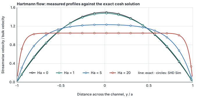
The strong check is not the distance from the curve. A profile can sit inside a generous tolerance and still be the wrong shape, and it can sit outside one and be the right shape scaled wrongly. So the harness recovers the Hartmann number from the measured shape by fitting, and prints it beside the one the dictionaries imply. That also checks the Ha formula: a missing square root or a factor of two would show as a fitted number tracking the expected one by a constant ratio across all three runs, which looks nothing like scatter.
| Ha asked for | Ha recovered from the shape | Difference | RMS deviation | Worst point |
|---|---|---|---|---|
| 0 | 0.0459574 | — | 0.0045 % | 0.0066 % |
| 1 | 1.0010256 | +0.103 % | 0.0046 % | 0.0080 % |
| 5 | 5.0011318 | +0.023 % | 0.0178 % | 0.0581 % |
| 20 | 20.2177495 | +1.089 % | 0.1658 % | 0.7664 % |
A second number says which profile it is, for a reader who is not going to plot anything: the velocity at half-way to the wall, divided by the velocity at the centre. That is 0.75 for a parabola and tends to 1 as the core flattens.
| Ha | u(a/2) / u(0) | u(0) / bulk | Exact u(0) / bulk |
|---|---|---|---|
| 0 | 0.756254 | 1.499875 | 1.499941 |
| 1 | 0.770985 | 1.476134 | 1.476193 |
| 5 | 0.932298 | 1.233115 | 1.233120 |
| 20 | 0.999115 | 1.052641 | 1.052632 |
The layer thickness behaves as the algebra says it should. Measured as where the profile first reaches 99 % of its centreline value, it is 4.6052 a/Ha at Ha = 20, 4.60525 at Ha = 50 and 4.6055 at Ha = 100 — a constant multiple of a/Ha, which is the statement that the layer thins in proportion to the field.
What this page does not establish
- Three Hartmann numbers is not a sweep to high field. Ha = 20 is the largest run here, and it is the one where the recovered number has begun to move.
- This is parallel plates, not a duct. The spanwise direction is one cell thick and empty. A real rectangular duct in a transverse field grows Shercliff layers on the side walls, whose profile is a different and not closed-form thing. The third direction was removed rather than approximated, which is what keeps the reference exact.
- The fluid is not a real liquid metal. ρ, ν and μ are left at 1 and the conductivity is lowered to put the case in the laminar, low-Rem regime, which sets the Hartmann number through B₀ alone. The staged case as the product writes it is air at 10 m/s, which is Re = 66 000 in a laminar solver and not a steady laminar anything.
- Nothing is established about the induced field itself. Everything measured here is the velocity profile. Bx was eliminated from the reference exactly, so the reference has nothing to say about it.
Repeat this yourself
Every case here is set up from the worked examples in the product, with no hand-editing of solver files — so you can run it, and get the same numbers. The free tier runs real cases up to 250,000 cells of fluids, or 100,000 nodes of solid, with no account needed to download and no time limit.
Other cases
- Turbulent plane channelThe only case here that tests turbulence modelling, against a DNS rather than an experiment — and it measures what a badly placed first cell costs you.
- Straight conductor, against AmpèreAmpère’s law is exact and the geometry is trivial, which is what makes the residual difference worth reporting rather than explaining away.
All validation cases · Written by the team building SHD Sim.