
Validation/Structural dynamics
Cantilever frequency response
The amplification at resonance is a ratio of two responses on one mesh, so the discretisation error cancels out of it. It is also the only quantity here that depends on the damping at all.
Why this case
The same steel cantilever as the deflection case and the modal case, carrying the same distributed load — but driven harmonically and swept through its first resonance at 35 frequencies.
Three quantities are checked, and they are limited by three different things:
- The static limit. Far below resonance a harmonic solve is the static solve, so the response must come back at wL⁴/(8EI).
- The resonant frequency, against the Euler–Bernoulli eigenvalue.
- The dynamic amplification at resonance — and this is the measurement.
| Physics | Harmonic structural response with Rayleigh damping |
|---|---|
| Material | Steel — E = 210 GPa, ν = 0.3, ρ = 7 850 kg/m³ |
| Applied | 10⁵ Pa distributed on the top face; damping ratio 0.02 at f₁ |
| Closed form | Euler–Bernoulli beam theory, and Q = 1/(2ζ) |
| Mesh | Tetrahedral, from Netgen — 1 383 elements |
| Agreement | Amplification at resonance within 0.211 % |
| Last run | 2026-08-27 |
Result
| Quantity | Closed form | Measured | Difference |
|---|---|---|---|
| Response below resonance | 8.928571 × 10⁻⁶ m | 9.148530 × 10⁻⁶ m | +2.464 % |
| Resonant frequency | 1 671.033 Hz | 1 637.613 Hz | −2.000 % |
| Amplification at resonance | 25.8517 | 25.9062 | +0.211 % |
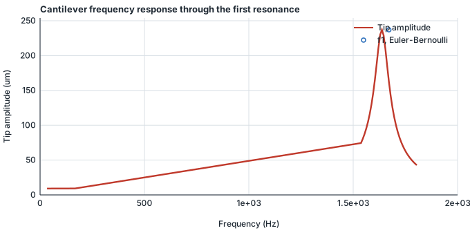
The −2.000 % on the resonant frequency is worth reading beside the modal case, which measures −2.13 % against the same formula on the same bar. Two different analysis types agreeing to 0.13 % about how far the beam idealisation sits from the solid.
Why the amplification is the measurement
The first two quantities are limited by a beam formula describing a three-dimensional solid. A few per cent is expected there and a tight tolerance would be a permanent failure.
The amplification is different in kind. It is a ratio of two responses on the same mesh — the peak divided by the static limit — so the discretisation error is in the numerator and the denominator alike and cancels. It lands at 0.211 % where the absolute deflection on that mesh is 2.46 %.
Why the reference is not simply 1/(2ζ)
A distributed load excites every mode. The static deflection is the sum over all of them; at resonance only the first is amplified. So the expected ratio is Q times the share of the static deflection the first mode accounts for.
For a cantilever under a uniform load that share is 101.34 % — slightly more than the whole of it, because the higher modes contribute with alternating signs and the second subtracts. It is computed from the mode shape rather than taken as a factor, so the reference stays closed-form and a reader can check it. It is not the 97 % figure quoted for a cantilever under a point load, and the two are easy to confuse.
The damping here is stiffness-proportional, so the damping ratio rises with frequency. The reference is therefore evaluated at the frequency the peak actually occurred at, not the one it was predicted for — using the predicted one instead moves the reference by 2 %, which is ten times the agreement being reported.
Repeat this yourself
Every case here is set up from the worked examples in the product, with no hand-editing of solver files — so you can run it, and get the same numbers. The free tier runs real cases up to 250,000 cells of fluids, or 100,000 nodes of solid, with no account needed to download and no time limit.
Other cases
- Cantilever natural frequencyThe modal companion to the cantilever deflection case: same beam, same closed form, a different analysis type.
- Cantilever step responseIt rings at 1634.5 Hz where the frequency-domain sweep on the same bar puts the resonance at 1637.6 — two different solvers agreeing to 0.19 % about a number neither was given.
All validation cases · Written by the team building SHD Sim.