
Draft. This manual is new and still growing. If something here does not match what you see in the software, the software is right — tell us and we will fix the page.
Your first simulation
The shortest path from opening the application to a result you can read. It uses a worked example, so there is nothing to import and nothing to draw.
Runs on the free tier.
Before you start
Two ideas make everything else make sense.
A case is one body and any number of studies of it. The geometry belongs to the case; the mesh, the physics and the run belong to a simulation inside it. That is why the setup tree has geometry once at the top and everything else repeated under each simulation — it is how you compare two meshes or two turbulence models on the same body without copying anything.
The application writes an ordinary OpenFOAM case. Nothing is hidden or proprietary. If you know OpenFOAM you can read every file it produces; if you do not, you never have to.
1. Open a worked example
From the home screen, press Worked example and choose External aerodynamics — streamlined hull from the menu. There are nine examples behind that button; this page follows the hull, which is air at 20 m/s over a towed body, and which arrives with its geometry already imported.
Four things to find before going further:
- The ribbon, across the top. Three tabs — Model, Geometry, Results — and every command lives on one of them. Meshing and running are on Model, which is the tab you start on.
- The setup tree, down the left. This is the workflow.
- The panel, which opens over the viewport when you select a tree row. It is where the settings are.
- The dock, along the bottom: Log, Residuals, Monitors, Case files, Problems.
The Model tab holds everything this page asks you to press. Its commands are grouped, and the group headings are the fastest way to find one:

2. Read the setup tree
The tree is the whole workflow, top to bottom, and it is worth two minutes now.
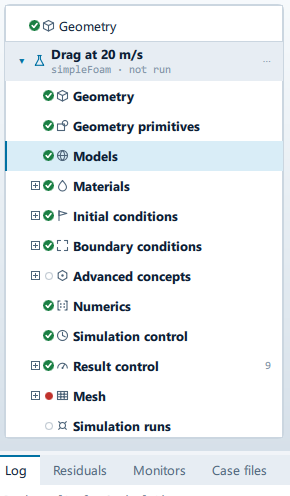
Mesh comes after the physics, not before it. That is deliberate: what to mesh follows from the domain and the boundary conditions, so the tree asks the physical questions first.
Each step shows a status dot, and the dots are computed from the case rather than ticked off by hand — a step goes green because the rules that check it are satisfied, not because you visited it.
The tree starts folded. Rows with a + have children, and those children are where a good deal of the setup lives. Mesh is the one to open first:
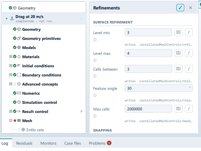
Advanced concepts is always present, even when the case has none — cell zones for MRF, AMI, overset, porous media and sources all live under it. The categories beneath it are hidden only where they cannot apply. It is available on every tier.
3. Look at what is already set
You do not need to change any of it, but look, because this is where the time goes on a real case:
- Models — the physics. For this case that is the analysis type, the time dependency, the algorithm and the turbulence model, which defaults to k-omega SST: the reasonable choice for external flow with adverse pressure gradients.
- Materials — the fluid, with its density and viscosity in real units.
- Boundary conditions — one entry per patch. Each knows which fields it needs, so you cannot leave a field unset without the Problems tab saying so.
- Simulation control — how long it runs and how often it writes.
The Problems tab in the dock is worth trusting. It reports what is wrong before you run, not after twenty minutes of solving.
4. Generate the mesh
Select Mesh and press Generate mesh — on the panel, or in the MESH group of the Model ribbon tab.
The mesh is built in the background and appears in the viewport when it finishes. Watch the Log tab in the dock if you want to see what it is doing.
Then open Mesh → Quality. It reports non-orthogonality, skewness and aspect ratio — the three numbers that decide whether a solver will struggle. A mesh that fails these does not usually announce itself by crashing; it announces itself by converging slowly to a slightly wrong answer, which is worse.
On the free tier the mesh is capped at 250,000 cells. The worked examples are sized to fit. Free is limited by scale rather than by physics: every analysis type, turbulence model, boundary condition and cell zone is available without a licence.
5. Run it
Select Simulation runs and press Start run. The RUN group on the Model ribbon tab does the same thing.
The dock fills with:
- the Log, streamed live,
- Residuals, plotted per equation,
- Monitors, if the case defines any.
Residuals falling steadily by several orders of magnitude is convergence. Flat residuals mean it has stopped improving. Rising residuals mean it is diverging, and the run will not recover on its own — stop it and see Troubleshooting.
You can keep working while it solves, and you can interrupt it three ways:
| What it does | |
|---|---|
| Stop gracefully | Finishes the current step, writes it, then stops |
| Kill | Ends the process now, behind a confirmation. The step it was part way through is lost |
| Continue | Not an interruption — after a finished or stopped run, it takes it on for more iterations |
There is a Pause button beside these, and on a solve it declines: suspending a running solver would corrupt its decomposition, so it logs that and tells you to Stop gracefully and then Continue instead. Pause is for the shorter jobs — meshing and the like.
6. Post-process
Post-processing belongs to a run, not to the simulation: a study with three runs would otherwise have three sets of results and no way to say which was meant. Expand Simulation runs → your run and the finished run carries Settings, Convergence plots, Solver Log, Solution Fields, Post-processing (with Boundary values under it) and Report.
Select Post-processing. The Results ribbon tab is now the live one, and its first two groups are the toolbox. FILTERS builds things in the viewport:
- Surface, Slice, Iso surface and Iso volume for the field distribution
- Streamlines, Vectors and Surface flow for direction
- Field calculator for a quantity the solver did not write
VIEW reads numbers back off what is there:
- Inspect point, Plot over line and Plot over path for numbers you can put in a document
- Statistics for the min, max, mean and integral of what is selected
Boundary values, for what is happening on each patch, is not on the ribbon: it is the tree row under Post-processing.
Start with a slice through the middle of the domain coloured by velocity. If that looks physically wrong — flow going the wrong way, a wake on the upstream side — the setup is wrong and no amount of further post-processing will fix it.
7. Report
Select Report under the finished run, then press Export PDF (A4).
The report gives results in engineering units, the split of drag into pressure and friction, and a verification checklist that states the threshold behind each verdict. Two sections are worth filling in before you export:
- Document control — the cover fields: title, author, revision, client.
- Snapshots — viewport captures you have saved, placed as numbered figures.
On the free tier the report is watermarked. Everything in it is real.
What to do next
The single most useful next step is to run the same case on a finer mesh. If the answer moves a lot, the first answer was mesh-dependent and was not an answer.
Two ways to get there. By hand: Duplicate the simulation from the ribbon, raise the mesh density on the copy, and run it. Or open the Study node, which generates the simulations for you — a sweep, a factorial design, one factor at a time, a Latin hypercube or a Sobol sensitivity.
Once the case holds two simulations, a Comparison row appears at case level. It puts them side by side and reports whether the result has converged on the mesh, and whether it depends on the turbulence model. Those are the two questions somebody will ask in a review, and a single run cannot answer either.