Flow in a pipe

At the end of this you will have a converged steady run of turbulent flow along a straight duct, a y+ figure that tells you whether the wall treatment was justified, and a pressure drop read off in engineering units.

Runs on the free tier. The analysis type is Incompressible, and the mesh is a plain block a few tens of thousands of cells in size.

Before you start

Read Your first simulation, and ideally Flow over a cylinder — this one moves faster over the steps that are the same.

Start from the bundled example. On the home screen, press Worked example and choose Internal flow - square duct. It arrives as a square duct of water with the physics already chosen, and no geometry to import.

There is a reason to start here rather than from New case: an internal-flow case has no body, so there is nothing for Auto wind tunnel to size the domain against. The bundled example carries its domain with it.

What is different about internal flow

Two things, and they drive everything below.

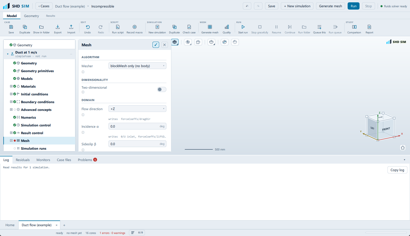
There is no body, so there is nothing to wrap a mesh around. The mesh is the domain. Under Mesh the Mesher is set to blockMesh only (no body) — its hint says exactly when that is right: a duct, a room, a manifold, where the fluid is the inside of something rather than the outside.

The walls are the boundary of the block, not a surface you imported. So the wind-tunnel patches are reused: inlet and outlet are the two ends along the flow axis, and farfield is everything else, set to Wall.

1. Geometry

Select Geometry — the row at the top of the tree, above the simulation heading, not the one under it. There is nothing to import and the pane says so — none - the block mesh is the domain.

Leave it alone and move on. This step exists in the tree because geometry belongs to the case, not because every case has some.

2. Mesh

Select Mesh.

Flow direction is set along the duct. This is not cosmetic: it decides which two faces of the block become inlet and outlet, and everything left over becomes farfield.

Base cell size is what sets the resolution across the passage. This is the one number that matters in an internal-flow mesh, and it is worth understanding why: the answer lives across the duct, not along it. A duct ten times longer than it is wide, meshed on a cell size scaled to its length, gets a handful of cells across the section and cannot represent a boundary layer at all.

The block underneath reports the domain size, the blockMesh divisions and the resulting cell count:

→  0.1 x 0.1 x 1 m
    blockMesh 12 x 12 x 120 = 0.02 M cells

Press Generate mesh. It is on this pane and also in the ribbon's MESH group, on the Model tab — which is where the commands live throughout: Start run and Continue in RUN, Comparison and Report in STUDY.

3. Refinements and Boundary layers

Both are effectively off for a blockMesh-only case, and correctly so. Refinements refines towards a surface, and there is no surface; Boundary layers grows prisms off one, likewise. The example sets the surface levels and the layer count to zero.

That is a real decision, not a shortcut, and it is what makes the next section matter.

4. Quality

Select Quality.

A pure block mesh should pass everything comfortably: non-orthogonality near zero, skewness near zero, no negative volumes. Layer coverage (body) will report 0% because there are no layers and no body patch — ignore that row here.

If a hex block does not pass these checks, something is wrong with the domain rather than with the meshing.

5. Models

Select Models.

Analysis type is Incompressible, Time dependency is Steady-state, Algorithm is SIMPLE. Fully developed duct flow settles down; there is no reason to integrate in time.

The setting to look at is Wall treatment, under Turbulence. It defaults to Wall functions, and the whole of the next section is about earning that choice.

Leave Model at k-omega SST.

6. Materials

Select Materials. The example uses Water (15 °C).

The derived block gives you the Reynolds number the case is actually at:

→  dynamic μ = …  Pa·s
    Re at … m/s over … m = …

Check it is where you think it is. A duct case set up in air by accident — which is what the defaults give you — has the right geometry, the right velocity and a Reynolds number an order of magnitude out, and nothing on screen looks wrong.

7. Initial conditions

Select Initial conditions.

For internal flow the pane's own warning is worth taking seriously: a uniform value everywhere is "fine for external flow; poor for internal flow with long ducts". Leave Track the inlet on so the domain starts at the inlet velocity rather than at rest — the flow then only has to develop its profile, not arrive in the first place.

Potential flow is the other option worth knowing about. It runs potentialFoam first to seed the velocity field, costs seconds, and removes the worst of the initial transient. On a duct it makes little difference; on anything with an obstruction it makes a lot.

8. Boundary conditions

Select Boundary conditions.

If the pane shows an amber block saying the patches do not match the generated mesh, press Use the mesh's patches. A block mesh has no body patch, and a condition left over for a patch the mesh does not have stops the solver on the first field it reads with an error that names a keyword rather than the problem.

You should end up with three:

Select inlet and check Intensity and Length scale under Turbulence. The block underneath converts them into the k, ω and ε the solver actually receives, which is the point of asking for the two you can estimate rather than the three you cannot. The pane suggests a length scale of about 7% of the body length and shows you what that is in metres.

Select farfield and confirm Wall motion is Stationary (no-slip) and Roughness is Smooth. A rough duct is a real thing and Sand-grain roughness is where you say so, but start smooth.

9. Result control — the y+ measurement

Select Result control.

Press + y+. Its description is the reason it is here: "wall distance in wall units - checks the layer resolution". This is not optional decoration. You chose Wall functions under Models, and wall functions are only valid over a range of y+; if the mesh puts the first cell centre outside that range, the turbulence model is being asked for something it cannot give, and nothing else in the run will say so.

Also press + Patch data. Set Patch to inlet and Operation to areaAverage, with Fields set to p. Add a second one on outlet the same way. The difference between them is the pressure drop, which is what an internal-flow case is usually run to obtain — the bundled example already has a patch-data item switched on for this reason.

Force coefficients mean nothing here. There is no body for them to be about.

10. Simulation control

Select Simulation control.

Iterations is the budget, not a promise: a steady run stops early if the residual targets under Numerics are met.

On the free tier the Cores list has one entry in it: the ladder is shortened by the licence rather than clamped afterwards. The hint on Cores states the efficient range — below about 10 k cells per core the communication costs more than the arithmetic saves — and on a mesh this size one core is the right answer anyway.

11. Run

Select Simulation runs — that is the node's name — and press Start run.

Watch Residuals. A steady internal-flow case should fall by several orders of magnitude and keep falling. Two failure signatures worth knowing:

• Residuals flatten early and high. The solution has stopped improving without converging. Usually the mesh, sometimes the numerics — try the Robust preset under Numerics.
• Residuals rise. It is diverging and will not recover. Stop it.

Watch Monitors for the two patch-data items. When the inlet and outlet pressures stop moving, the pressure drop has converged — which is a better test of convergence than the residuals are, because it is the quantity you actually want.

12. Post-processing

Post-processing hangs under the run rather than beside the setup steps: Simulation runs → <your run> → Post-processing, and it appears only once that run has finished. Selecting it switches the ribbon to the Results tab.

Press Show results.

Under Ready-made views, press Mesh adequacy. It builds a surface coloured by y+ and a slice, which is the direct answer to "was the wall treatment justified".

Read the y+ colour bar. With wall functions you want the wall values within the range the Boundary layers pane names — between 30 and 300. Below that range the wall function is being applied where the mesh could have resolved the layer properly, and it will be wrong; far above it, the first cell is out in the free stream and the wall shear is a guess.

If y+ is out of range, the fix is in Mesh: change Base cell size, or add prism layers under Boundary layers with a Target y+ in range, and re-mesh. It is not something you can correct after the fact.

Then use Sample along a line under Plot over line. Set the ends across the duct rather than along it, choose U, and you get the velocity profile. Press Export CSV to take the numbers away.

13. Boundary values

Select Boundary values, which sits under Post-processing under the same run.

Choose a Patch and a Field and press Measure, or press Every wall to do them all. This gives you the area, the mean and the integral on each patch after the fact — the same numbers the patch-data items recorded during the run, from the written result rather than from the monitor files.

Export as CSV puts them somewhere you can use them.

What you should see

A velocity profile that is flat across the middle and steep at the walls — the turbulent profile, not the parabola of laminar flow. A pressure that falls linearly along the duct once the flow is developed. And a y+ on the walls that sits inside the wall-function range along most of the duct.

Three things that mean it is wrong: a parabolic profile at a Reynolds number in the tens of thousands (check the turbulence model is not Laminar), a pressure that rises along the flow, or y+ in the single digits with Wall functions selected.

What to try next

• Mesh independence study — the pressure drop you just measured is a number, but it is not yet a result.
• External aerodynamics for the opposite case: a body with flow around it rather than a passage with flow through it.
• Conjugate heat transfer if the duct wall conducts and you care what it does.